Low-Rank Adaptation of Large Language Models (LoRA)

Overview

LoRA (Low-Rank Adaptation) is a parameter-efficient fine-tuning technique that enables adaptation of large language models to specific tasks or domains without modifying the entire model. Introduced by Hu et al. (Hu et al. 2021), LoRA addresses the computational and storage challenges of fine-tuning models with hundreds of billions of parameters, such as GPT-3 with 175 billion parameters.

Traditional fine-tuning approaches require updating all model parameters, which becomes computationally prohibitive for large models. LoRA instead freezes the pre-trained model weights and injects trainable rank decomposition matrices into each layer of the Transformer architecture, greatly reducing the number of trainable parameters for downstream tasks.

The Problem

As language models scale to hundreds of billions of parameters, full fine-tuning becomes increasingly challenging:

Storage: Each fine-tuned model requires storing all parameters, making it expensive to maintain multiple task-specific models
Memory: Fine-tuning requires substantial GPU memory to store gradients and optimizer states for all parameters
Deployment: Switching between different fine-tuned models requires loading entirely different model checkpoints

For GPT-3 175B, deploying independent instances of fine-tuned models, each with 175B parameters, is prohibitively expensive. LoRA addresses these challenges by reducing the number of trainable parameters by up to 10,000 times while maintaining comparable performance.

How LoRA Works

Low-Rank Decomposition

LoRA is based on the observation that weight updates during fine-tuning often have a low “intrinsic rank”—meaning the changes can be represented efficiently using low-rank decompositions. For a pre-trained weight matrix W_0 \in \mathbb{R}^{d \times k}, LoRA constrains its update by representing it with a low-rank decomposition:

\Delta W = BA

where B \in \mathbb{R}^{d \times r}, A \in \mathbb{R}^{r \times k}, and the rank r \ll \min(d, k).

During training, W_0 is frozen and does not receive gradient updates, while A and B contain trainable parameters. The modified forward pass becomes:

h = W_0 x + \Delta W x = W_0 x + BA x

Understanding the Concept with a Simple Example

Think of it this way: instead of changing a huge matrix directly, we break the changes into two smaller matrices that, when multiplied together, give us the same result. It’s like factorising a number—instead of working with 100 directly, we can work with 10 × 10.

Let’s see this in action with a concrete example. We’ll start by setting up the dimensions:

import numpy as np

# Set up dimensions for our example
# In real Transformers, these could be 768, 1024, or even 12288
d = 768  # Output dimension (how many features come out)
k = 768  # Input dimension (how many features go in)
r = 4    # Rank - the "compression factor" (much smaller than d and k)

The original matrix would be: 768 × 768 = 589824 parameters.

LoRA will use rank r = 4 (much smaller!)

Now, let’s create the original pre-trained weight matrix. This represents what the model learned during initial training, and we’ll keep it frozen (unchanged):

# The pre-trained weight matrix - this stays frozen (unchanged)
W_0 = np.random.randn(d, k) * 0.02

The W_0 shape is (768, 768) and W_0 has 589824 parameters (this is what we’d normally update)

Instead of updating all those parameters, LoRA creates two much smaller matrices. Here’s the key insight: when we multiply these two small matrices together, we get a matrix the same size as W_0, but we only need to train the small ones:

# Create the two LoRA matrices
# B is tall and thin: (d × r) = (768 × 4)
B = np.zeros((d, r))  # Starts as all zeros

# A is short and wide: (r × k) = (4 × 768)  
A = np.random.randn(r, k) * 0.02  # Starts with small random values

The B shape is (768, 4) and B has 3072 parameters. The A shape is (4, 768) and A has 3072 parameters. The total LoRA parameters are 6144

When we multiply B and A together, we get a matrix the same size as W_0, but notice how many fewer parameters we’re actually training:

# Multiply B and A to get the update matrix
# (768 × 4) @ (4 × 768) = (768 × 768)
Delta_W = B @ A

The \Delta_W shape is (768, 768) and \Delta_W has 589824 values, but we only trained 6144 parameters!

At the start, \Delta_W is all zeros.

The magic is in the parameter count. Let’s compare:

# Count the parameters
params_full = d * k           # Full fine-tuning: update everything
params_lora = d * r + r * k   # LoRA: only update B and A
reduction = params_full / params_lora

Full fine-tuning: 589824 parameters. LoRA fine-tuning: 6144 parameters. This is a reduction of 96.0× fewer parameters to train!

Now let’s see how this works during the forward pass. The input goes through both the frozen weights and the LoRA update:

# Create a sample input
x = np.random.randn(k, 1)

The input x shape is (768, 1).

# Standard approach: just use W_0
h_standard = W_0 @ x

# LoRA approach: use W_0 (frozen) + BA (trainable)
h_lora = W_0 @ x + (B @ A) @ x
# This is equivalent to: h_lora = W_0 @ x + Delta_W @ x

The standard output shape is (768, 1) and the LoRA output shape is (768, 1). The shapes match: True. The key advantage: after training, we can merge everything into a single matrix for faster inference:

# After training, merge the weights for efficient inference
W_merged = W_0 + B @ A
h_merged = W_merged @ x

After merging, we have a single matrix again. The merged matrix shape is (768, 768) and the same result as LoRA.

Demonstrating That LoRA Actually Works

To show that LoRA can learn effectively, let’s create a simple task: we’ll train LoRA to approximate a target transformation. We’ll compare the results with and without LoRA to see that it actually learns the task.

First, let’s set up a simple learning task:

# Set up a simpler example for demonstration
d_small = 64
k_small = 64
r_small = 4

# Create a target transformation we want to learn
np.random.seed(42)
W_target = np.random.randn(d_small, k_small) * 0.1

# Create pre-trained weights (different from target)
W_0_small = np.random.randn(d_small, k_small) * 0.02

# The task: learn to transform W_0 to approximate W_target
# In real scenarios, this would be learning a task-specific adaptation

Now let’s train LoRA to learn this transformation:

# Initialise LoRA matrices
B_small = np.zeros((d_small, r_small))
A_small = np.random.randn(r_small, k_small) * 0.02

# Simple gradient descent training
learning_rate = 0.01
n_steps = 1000
losses = []

for step in range(n_steps):
    # Generate random input
    x_train = np.random.randn(k_small, 1)
    
    # Forward pass: W_0 (frozen) + BA (trainable)
    y_pred = W_0_small @ x_train + (B_small @ A_small) @ x_train
    
    # Target output
    y_target = W_target @ x_train
    
    # Compute loss
    error = y_pred - y_target
    loss = np.mean(error ** 2)
    losses.append(loss)
    
    # Compute gradients (simplified - in practice, use autograd)
    # Gradient for B: dL/dB = error @ (A @ x).T
    grad_B = error @ (A_small @ x_train).T
    # Gradient for A: dL/dA = B.T @ error @ x.T
    grad_A = B_small.T @ error @ x_train.T
    
    # Update only B and A (W_0 stays frozen!)
    B_small -= learning_rate * grad_B
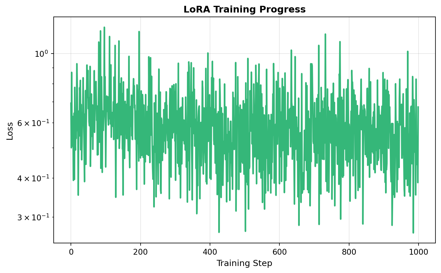
    A_small -= learning_rate * grad_A

The initial loss is 0.6937475547880915 and the final loss is 0.6743411926046452. The loss reduction is 1.0287782540889858×.

Let’s compare the results. We’ll measure how well LoRA approximates the target compared to using just the frozen weights:

# Test on new data
x_test = np.random.randn(k_small, 10)

# Output with just frozen weights (no adaptation)
y_frozen = W_0_small @ x_test

# Output with LoRA adaptation
y_lora = W_0_small @ x_test + (B_small @ A_small) @ x_test

# Target output
y_target_test = W_target @ x_test

# Measure errors
error_frozen = np.mean((y_frozen - y_target_test) ** 2)
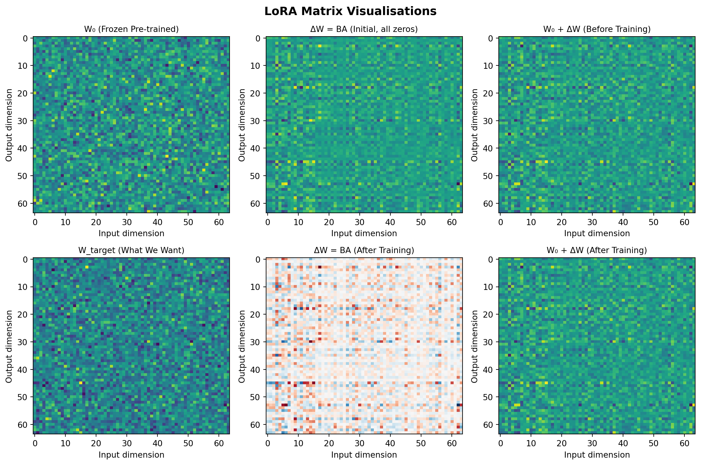
error_lora = np.mean((y_lora - y_target_test) ** 2)

The error with frozen weights only is 0.7678328463678933 and the error with LoRA adaptation is 0.6283674537204684. The improvement is 1.2219487846190495× better. Now let’s visualise the matrices to see what LoRA learned:

Let’s also plot the training progress:

Visual Summary:

Instead of updating all 589,824 parameters in W_0, LoRA only trains 6,144 parameters in B and A—a 96× reduction! As the demonstration above shows, LoRA can effectively learn task-specific adaptations while using far fewer parameters, making fine-tuning large models feasible on consumer hardware.

Initialisation and Scaling

LoRA uses a random Gaussian initialisation for A and zero initialisation for B, ensuring that \Delta W = BA is zero at the beginning of training. The update is then scaled by \frac{\alpha}{r}, where \alpha is a constant. This scaling helps reduce the need to retune hyperparameters when varying r.

Application to Transformers

In the Transformer architecture, there are four weight matrices in the self-attention module (W_q, W_k, W_v, W_o) and two in the MLP module. LoRA is typically applied to the attention weights, with empirical studies showing that adapting both W_q and W_v provides the best performance for a given parameter budget.

Key Advantages

Parameter Efficiency

LoRA dramatically reduces the number of trainable parameters. For GPT-3 175B with r=4 and only query and value projection matrices adapted, the checkpoint size is reduced by roughly 10,000× (from 350GB to 35MB). This makes fine-tuning feasible on consumer hardware that would otherwise be incapable of handling such large models.

No Inference Latency

Unlike adapter layers, which introduce additional depth and sequential processing, LoRA can be merged with the frozen weights during deployment. By explicitly computing and storing W = W_0 + BA, inference proceeds as usual with no additional latency compared to a fully fine-tuned model.

Memory Efficiency

For large Transformers trained with Adam, LoRA reduces VRAM usage by up to 2/3, as it doesn’t need to store optimizer states for frozen parameters. On GPT-3 175B, VRAM consumption during training is reduced from 1.2TB to 350GB.

Task Switching

A pre-trained model can be shared and used to build many small LoRA modules for different tasks. Task switching is efficient—simply swap the small A and B matrices rather than loading entirely different model checkpoints. This allows maintaining one base model with numerous lightweight adapters for different applications.

Training Speed

LoRA achieves a 25% speedup during training on GPT-3 175B compared to full fine-tuning, as it doesn’t need to calculate gradients for the vast majority of parameters.

Empirical Findings

Optimal Rank

Surprisingly, LoRA performs competitively with very small ranks. For GPT-3 175B, a rank as small as r=1 or r=2 suffices for many tasks, even when the full rank dimension is as high as 12,288. This suggests that the adaptation matrix \Delta W has a very low intrinsic rank.

Weight Matrix Selection

Empirical studies show that adapting both W_q and W_v yields the best performance for a given parameter budget. Adapting only W_q or W_k results in significantly lower performance, while adapting all four attention matrices (W_q, W_k, W_v, W_o) provides marginal improvements.

Relationship to Pre-trained Weights

Analysis of the learned adaptation matrices reveals that \Delta W amplifies features that are important for specific downstream tasks but were not emphasised in the general pre-training model. The adaptation matrix has a stronger correlation with W compared to a random matrix, but instead of repeating the top singular directions of W, \Delta W amplifies directions that are not emphasised in W.

Comparison with Other Methods

Adapter Layers

Adapter layers introduce additional depth to the model, requiring sequential processing that adds inference latency. In online inference scenarios with small batch sizes, adapters can introduce 20-30% latency overhead. LoRA avoids this by allowing weight merging during deployment.

Prefix Tuning

Prefix tuning optimises continuous prompts by reserving part of the sequence length for adaptation. This necessarily reduces the sequence length available for task tokens. LoRA doesn’t reduce available sequence length and is generally easier to optimise.

Full Fine-tuning

While full fine-tuning provides maximum expressiveness, it requires updating and storing all model parameters. LoRA achieves comparable performance with a fraction of the parameters, making it practical for large-scale deployment scenarios.

Implementation

LoRA can be applied to any dense layers in neural networks, though it’s most commonly used with Transformer attention layers. The technique is orthogonal to many prior methods and can be combined with approaches like prefix-tuning for potentially improved performance.

The original implementation is available at Microsoft’s LoRA repository, which provides integration with PyTorch models and implementations for RoBERTa, DeBERTa, and GPT-2.

Applications

LoRA has become widely adopted in the LLM community for:

Domain Adaptation: Adapting general-purpose models to specific domains (e.g., medical, legal, scientific)
Task-Specific Fine-tuning: Creating specialised models for specific tasks (e.g., summarisation, question answering)
Multi-Task Deployment: Maintaining a single base model with multiple lightweight adapters for different applications
Resource-Constrained Environments: Enabling fine-tuning on consumer hardware or with limited computational resources

Limitations

LoRA has some limitations:

It’s not straightforward to batch inputs to different tasks with different A and B matrices in a single forward pass if weights are merged
The optimal rank and which weight matrices to adapt may require task-specific tuning
For tasks that differ significantly from pre-training (e.g., different languages), full fine-tuning or higher ranks may be necessary

References

Hu, Edward J., Yelong Shen, Phillip Wallis, Zeyuan Allen-Zhu, Yuanzhi Li, Shean Wang, Lu Wang, and Weizhu Chen. 2021. “LoRA: Low-Rank Adaptation of Large Language Models.” arXiv Preprint arXiv:2106.09685.